Note

This is the documentation for the latest development branch and may refer to features that are not available in released versions. If you are looking for the documentation for a specific release, use the drop-down menu on the left and select the desired version.

K230 ISP Image Tuning Guide

Note: This document focuses on ISP full tuning methods and module parameter descriptions. If you are currently only doing BLC/LSC/CC calibration operations, please also read: how_to_calibrate_isp.md.

K230 ISP Image Tuning Overview

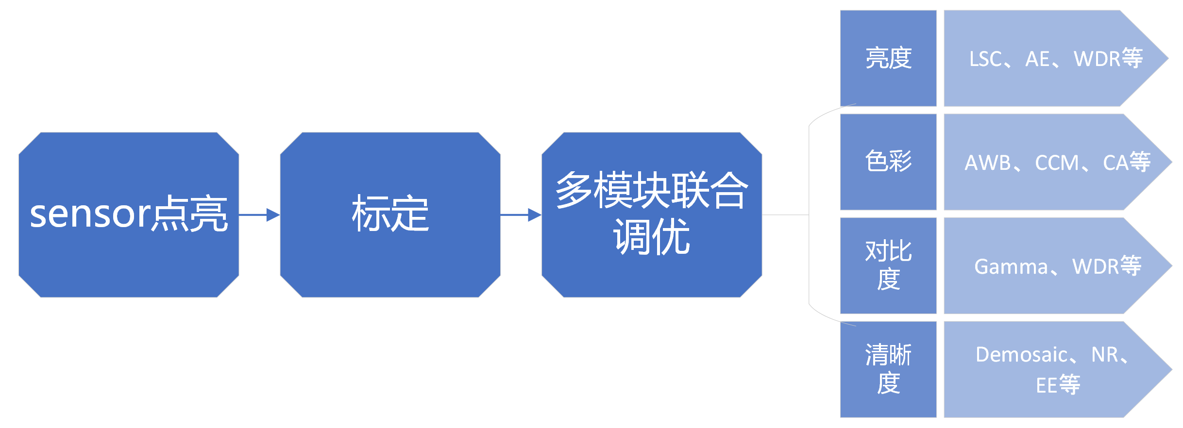
When performing image tuning, brightness, color, contrast, and sharpness are our main concerns. Through the calibration of the sensor and lens and the joint tuning of ISP sub-modules, the overall brightness of the image should be reasonable, the color reproduction in the image should be accurate, the image sharpness should be good, there should be no obvious noise, the image contrast should be high, and the overall appearance should be relatively transparent.

The overall image tuning process is shown in the figure below:

The K230 ISP pipeline is shown in the figure below:

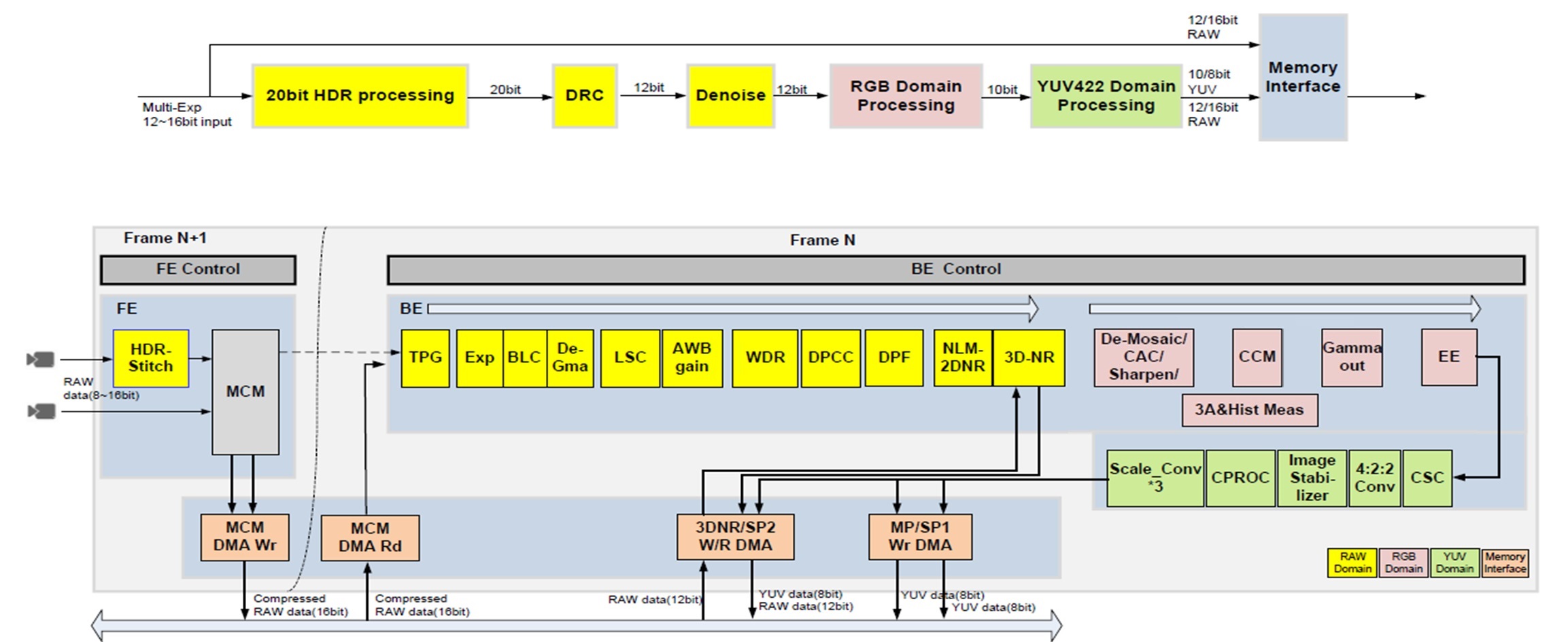
Please note:

• In K230 HDR mode, the K230 CSI (Camera serial interface) module does not support sensor data mode where Hsync comes before Vsync, and the Vsync of each frame (L/S/VS) cannot overlap when pulled high (valid data output).

• When enabling TNR in 3DNR, the ISP requires that the sensor Hblank cannot be less than 180 pixel clocks (recommended to be set to no less than 256 pixel clocks). Recommendation: Frame length – Active lines >= 92 lines.

Calibration

Overview

Use the calibration tool (K230ISPCalibrationTool.exe) to complete the parameter calibration functions for the six ISP modules: BLC, LSC, CC, AWB, Noise Profile, and CAC.

The calibration order of the modules is as follows:

Before using the calibration tool (K230ISPCalibrationTool.exe), users need to pre-install MATLAB Runtime (R2023a). Download link: https://ssd.mathworks.com/supportfiles/downloads/R2023a/Release/0/deployment_files/installer/complete/win64/MATLAB_Runtime_R2023a_win64.zip

The main interface of the calibration tool is shown in the figure below.

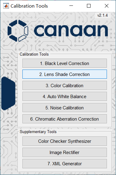
Click the corresponding module button to jump directly to the calibration interface of each module to start calibration.

Black level correction

The principle and significance of black level calibration

When the analog signal is very weak, it may not be converted by A/D, resulting in loss of image details when the light is very dim. Therefore, the Sensor will give a fixed offset to the analog signal before A/D conversion to ensure that the output digital signal retains more image details. The black level correction module determines the specific value of this offset through calibration. Subsequent ISP processing modules need to subtract this offset value first to ensure the linear consistency of the data. If the black level parameters of the sensor are not obtained in advance, or more accurate black level values are required, black level calibration should be performed.

Capturing RAW images for black level calibration

When performing black level calibration, the steps to capture RAW images are as follows:

1. Place the module in a completely dark environment (such as covering the lens with a black cloth) to ensure no light enters the sensor;

2. Set the sensor’s exposure mode to manual mode;

3. Capture 12 RAW images under different combinations of Gain values (1x, 2x, 3x, 4x) and different integration times (0.01ms, 0.02ms, 0.03ms);

4. Save them to a folder according to the naming convention. The folder naming format: Gain_4_T_0.03 (Gain_4_T_0.03 indicates exposure gain = 4, exposure time = 0.03s), and other exposure time and Gain naming formats follow the same pattern.

Starting calibration with the calibration tool

After clicking “Black level correction” on the main interface, the tool will pop up the dialog box as shown in the figure.

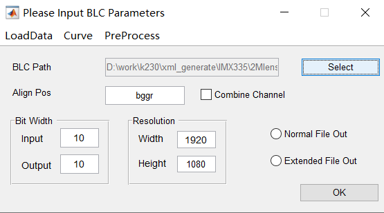
Operation steps:

1. Click the “Select” button to choose the saved RAW image folder;

2. “Align Pos” text box: Fill in the bayer pattern of the RAW image;

3. Set the input and output Bit Width;

4. Set the resolution: the width and height of the image;

5. Click the “OK” button to perform calibration.

Among them:

1. Combine Channel text box: If checked, it indicates that the BLC obtained by the user is the measured value after combining the four channels R, Gr, Gb, and B.

2. Normal File Out / Extended File Outy: If Normal File Out is checked, it indicates that the output is blc_para.txt; if Extended File Out is checked, it indicates that the BLC of R, Gr, Gb, and B channels will be output separately according to different exposure times and Gains.

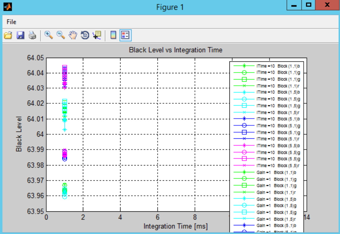
After calibration is completed, the Black Level vs Integration Time chart is shown in the figure below.

Lens shading Correction

Basic Principles and Significance of LSC Calibration

The purpose of LSC calibration is to eliminate the vignetting caused by uneven optical refraction of the lens. In the Lens shading phenomenon, the brightness attenuation from the central target point to the corners follows the cosine fourth power law. The calibration results can effectively reflect the brightness attenuation trend, using a 32x16 grid to store the calibration results, and then restoring the brightness of each area of the image to the brightness of the target point. LSC calibration includes luma shading and color shading calibration. Because the color shading characteristic curves differ under different color temperatures, to meet the color shading correction requirements under different color temperatures, LSC calibration needs to be performed at different color temperatures.

LSC Calibration RAW Image Capture

Precautions before capturing RAW images:

• Adjust the AE target brightness settings so that the average brightness of the image center is about 80% of the maximum value (e.g., 8bit: 255)

• The light source environment for the LSC capture object must be a light source with flat and uniform brightness distribution, and the capture object must remain smooth and texture-free. Therefore, the DNP light box can be selected as the scene for capturing RAW images for LSC calibration.

When performing LSC calibration, the steps to capture RAW images are as follows:

1. Control the device’s lens to align with the target area of the DNP light box, and ensure that the environment is not disturbed;

2. Turn on the DNP light box, switch the color temperature light source to D65, and set the light box to an appropriate illuminance;

3. Capture a RAW image;

4. Switch the DNP light box’s light source (D50, TL84, F12, A), and repeat steps 2-3.

Using the Calibration Tool to Start Calibration

After clicking “Lens Shade correction” on the main interface, the tool will pop up the dialog box as shown in the figure.

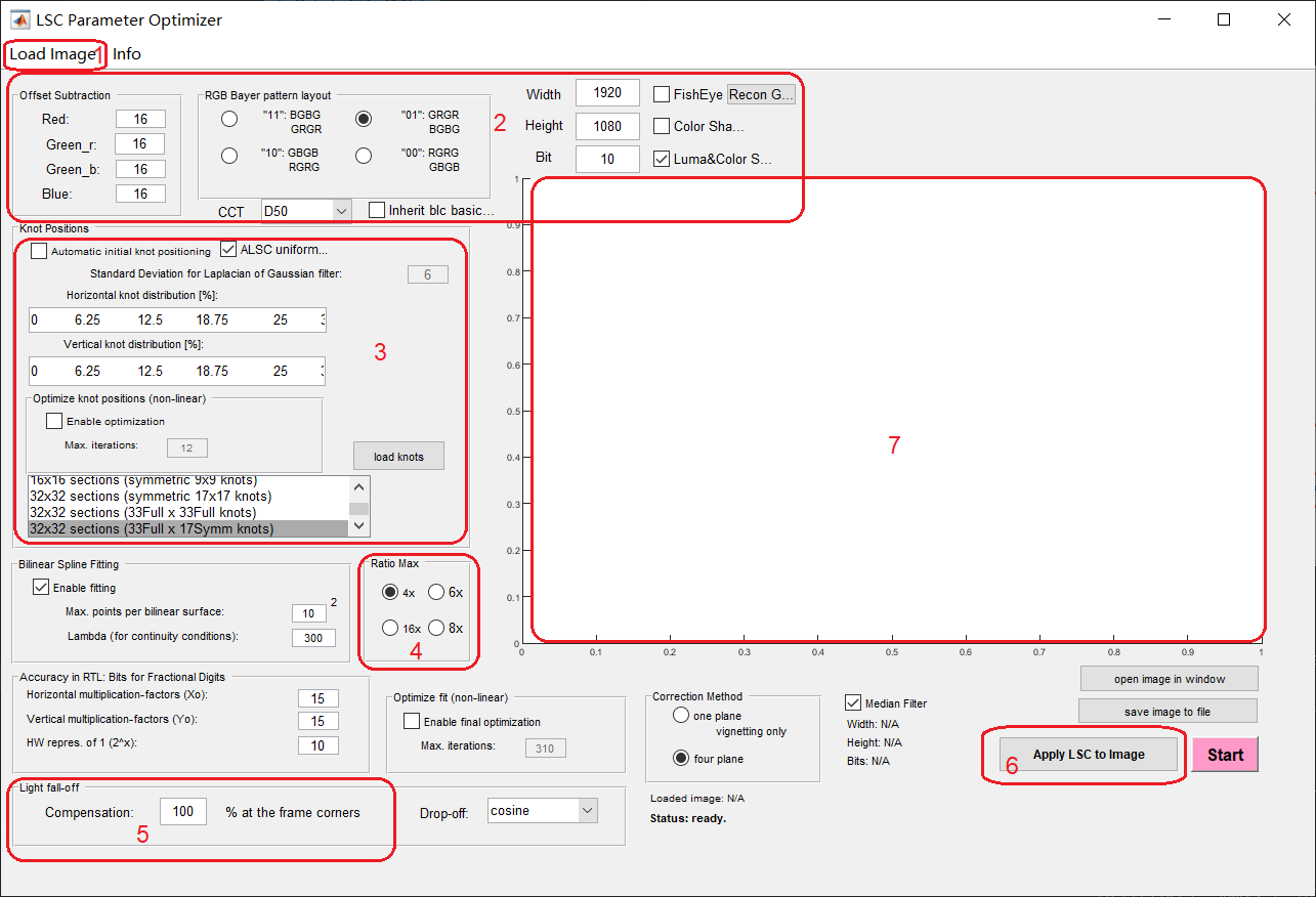
Specific operation steps:

1. In area 2, select the bayer pattern order of the RAW image, fill in the image width, height, and bit width, select the required type of lsc correction (Color Shading or Luma&Color Shading), select the corresponding color temperature light source in the CCT drop-down bar, and fill in the Black Level Offset values of each channel in the offset Subtration column;

2. Click the “load image” button in area 1 to import the RAW image to be calibrated;

3. Area 3 is for lsc grid node settings. First determine the number of grids. K230 ISP LSC hardware statistics is a 32x16 grid, so you can select “33Full x 17Symm knots” for calibration; if you plan to use the ISP ALSC function, check “ALSC uniform…”; if “Automatic initial knot positioning” is checked, the ALSC function cannot be enabled in auto.json.

4. Area 4 allows you to select the maximum calibration ratio for the center/edges;

5. Area 5 allows you to set the corner compensation ratio (for example, if set to 80%, it means the brightness of the corners after calibration needs to be 80% of the center brightness);

6. Other settings can remain at the default configuration;

7. Click “Start” to begin calibration and save the LSC data;

8. Area 6 allows you to select the calibrated LSC data to apply to the image, preview the calibration effect, and click “save image to file” to save the Png images under each light source.

Note: When setting the compensation ratio in step 5, it should be determined based on the severity of the lens shading. When the lens shading is very severe, the compensation gain for the four corners of the image is very large, which can easily lead to increased noise at the four corners. In this case, the compensation ratio should be reduced to achieve the goal of optimizing the noise at the four corners.

Color Correction

CCM Calibration Principle

The principle of CCM calibration is to compare the actual color information of the 24-color card patches collected by the sensor with their expected values, and calculate a 3x3 CCM matrix. The 3x3 matrix of CCM converts the sensor’s color space to the sRGB standard color space.

CC Calibration RAW Image Collection

During CC calibration, the steps to collect RAW images are as follows:

1. The 24-color card can be placed on the inner wall of a standard light box (the lens faces the color card to collect RAW images) or the 24-color card can be placed at the bottom of the light box (the lens is at a 45-degree angle to the 24-color card to collect RAW images);

2. Turn on the standard light box, select the D65 light source, and adjust the light box illuminance;

3. Adjust the distance and position of the lens to the 24-color card to ensure that the 24-color card occupies about 2/3 of the image range;

4. Adjust the AE target brightness setting to ensure the average brightness of the RAW image is around 50;

5. Collect one RAW image;

6. Switch the light source (D50, TL84, F12, A) and repeat step 5;

7. Keep the lens position unchanged, remove the 24-color card, and then collect RAW images of the gray wall background on the inside of the light box under 5 light sources.

Start Calibration with the Calibration Tool

After clicking “Color Correction” on the main interface, the tool will pop up the dialog box as shown in the figure.

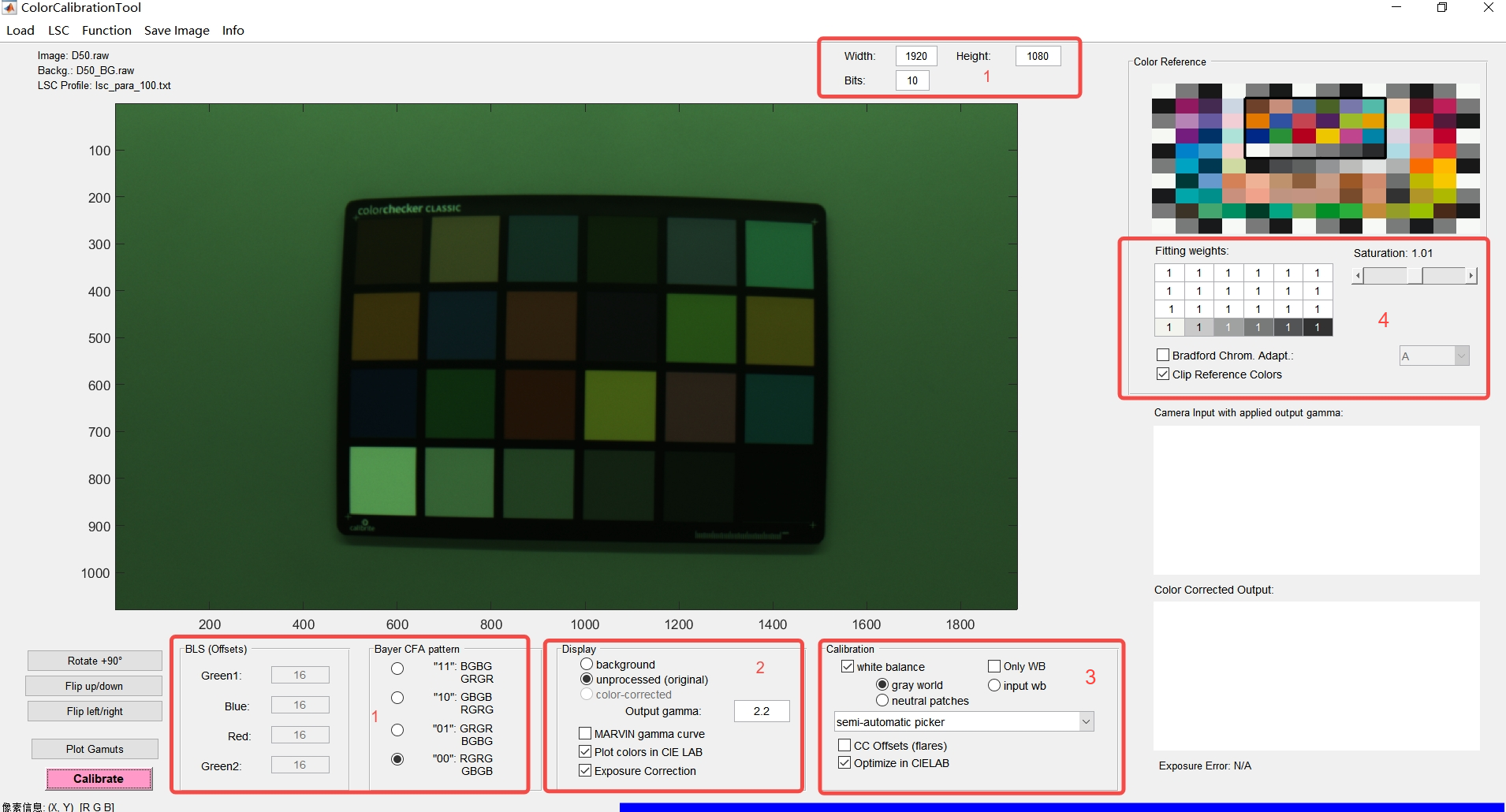
The specific operation steps are as follows:

1. Set the RAW image width and height, bit width, Black level Offset, and bayer pattern in area 1;

2. Click the “Load” menu to import the color patch reference file CC_Standard.cxf in sequence (Load sRGB References, which is located in the Canaan.Calibration.Samples\Data\ directory of the calibration tool), the 24-color card RAW image (Load Color Checker Image), and the gray wall background RAW image (Load Background Image);
   To import the reference color patch, in addition to importing CC_Standard.cxf through “Load sRGB References”, you can also obtain the customer-defined reference color patch Lab values through “Load Lab-Customer References” under the “Load” menu; or through “Load References Image” under the “Load” menu, load the reference color patch image, then select “Select Reference Color Check” under the “Function” menu, and by moving the mouse to control the crosshair, let it be located at the center of the four color blocks at the upper left, upper right, lower left, and lower right corners of the given color patch in sequence, and click the mouse in turn to complete the specification of the reference color patch area.

3. Click the “LSC” button to import the calibrated LSC parameter file;

4. Configure calibration parameters;

   • Set gamma

   • Check CIELAB reference

   • Configure 24 color block weights

   • Set preferred light source

   • Set output saturation, default is 1

5. In the drop-down key of area 3, select the way to select the 24 color blocks (there are three modes: automatic, semi-automatic, and manual);
   In semi-automatic mode, by moving the mouse to control the crosshair, let it be located at the center of the four color blocks at the upper left, upper right, lower left, and lower right corners of the color patch image in sequence, and click the mouse in turn to complete the specification of the reference color patch area.

6. Click “Caibrate” to start calibration.

Auto White Balance

Basic Principles and Significance of AWB Calibration

AWB calibration involves calculating the optimal Planck fitting curve and color temperature fitting curve based on the sensor’s white point characteristics (R/G, B/G) under several standard light sources. The purpose of AWB calibration is to enable the camera to automatically recognize and adapt to various color temperature light source conditions, ensuring accurate reproduction of white and other colors in images.

Using the Calibration Tool to Start Calibration

After clicking “Auto White Balance” on the main interface, the tool will pop up the dialog box as shown in the figure.

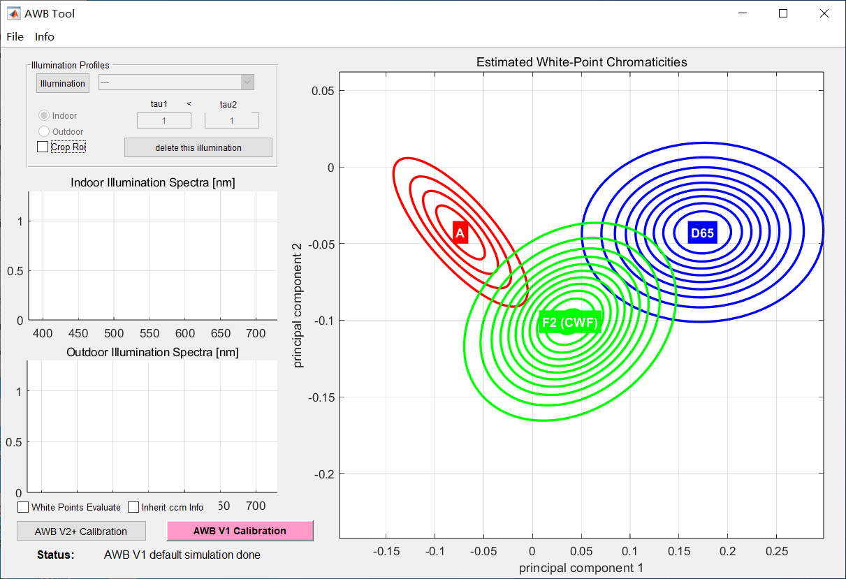
The specific operation steps are as follows:

1. Click the “file” button to import the sensor spectral sensitivity file, as shown in the figure below;

   

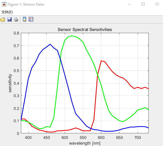
   Note: If the user does not have the spectral sensitivity file of their own sensor, the default OV2775_sensitivity.txt in the tool package (located in the Canaan.Calibration.Samples\Data\ directory of the calibration tool) can be used. Because AWB calibration no longer depends on the sensor spectral sensitivity file now, but to avoid affecting subsequent operations, importing any sensor spectral sensitivity file is sufficient.

2. Click the “illuination” button to import the light source file CIE_Illuminants.cxf (located in the Canaan.Calibration.Samples\Data\ directory of the calibration tool), and select the light sources to be calibrated (at least 3), as shown in the figure. Click the “OK” button, and the spectral distribution of each light source will be displayed on the left side as shown in the figure, and use the drop-down key to classify each light source into indoor light sources and outdoor light sources.

   

   

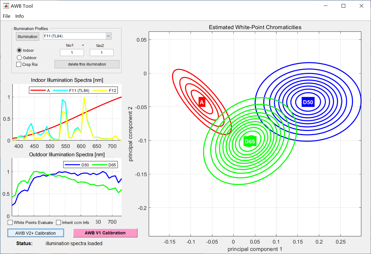
3. Click the “AWB V2+ Calibration” button (in the old version of the calibration tool, please click the “Start Calibration” button). According to the red box shown in the figure, select the parameter files of each light source generated by CC calibration;

   

4. Check the “White Points Evalute” box and select an image for white point estimation;

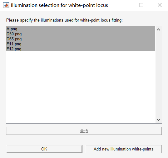
5. Click the “Gain Region Modifier” button to select the png images of each light source saved in LSC calibration, as shown in the figure, and click “OK” to enter the next step;

   

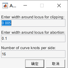
6. Define the starting range size of the gain polygon, as shown in the figure, click the “OK” button to enter the next step;

   

7. Manually adjust the range of the orange box (near white area) and the black box (all points falling within the black box are identified as white points) through the buttons in the red box area. The range of the black box should include all selected light source white points, as shown in the figure. Save the data. If the test fails, readjust the range of the polygon.

   

Calibration of AWB Parameter K_Factor

In the AWB algorithm, the environment is judged as outdoor if: Exp*K_Factor <=0.12 (Exp is the exposure amount).

For example, with 2000 lux as the illuminance division point between outdoor and transition environments, obtain the exposure value (ET * gain) corresponding to this illuminance, then it can be calculated: K_Factor = 0.12 / (ET*gain).

Noise Calibration

Principle and Significance of Noise Profile Calibration

Noise Profile calibration involves quantitatively measuring and describing the noise characteristics generated by the sensor under different conditions. This is because when sensors operate under different lighting, temperature, or ISO settings, they produce different types and magnitudes of noise. Understanding these noise characteristics is key to performing effective noise reduction or correction.

Capturing RAW Images for Noise Profile Calibration

During CC calibration, the steps for capturing RAW images are as follows:

1. Place the black-and-white gradient test card on the inner wall of the standard light box, turn on the light box and select the D50 color temperature light source;

2. Turn off AE and switch to manual exposure mode, then capture two groups of RAW images, 30 images per group;

   • Bright group: Adjust the light box brightness, keep the exposure time, keep gain at 1x unchanged, so that the black area of the gradient card is at the middle gray value;

   • Dark group: Adjust the light box brightness, keep the exposure time, keep gain at 1x unchanged, so that the white area of the gradient card is at the middle gray value.

Starting Calibration with the Calibration Tool

After clicking “Noise Calibration” on the main interface, the tool will pop up the dialog box as shown in the figure.

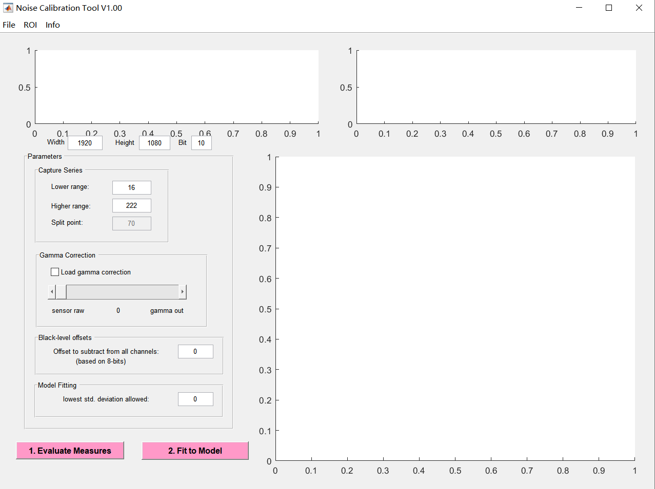
The specific operation steps are as follows:

1. Set the width, height, bit width, and Black level Offset of the RAW image;

2. Click the “flie” button to import the bright and dark groups of RAW image series;

3. Click the “ROI” button to set the ROI of the image;

4. Adjust parameters. For the Lowlight histogram, take the histogram region from the Lower range to the Split point; for the Highlight histogram, take the histogram from the Split point to the Higher range. The combined region of the two should basically cover all values from 0 to 255 (8-bit width). For the selection of the Split point and high range values, the reserved regions of highlight and lowlight should conform to a Poisson distribution. If black level offset is set, then Lower range >= black level;

5. Gamma correction and Model Fitting do not need to be set;

6. Click “Evaluate Measures”;

7. Then click “Fit to Model” to complete the Noise calibration and save the result.

Chromatic Aberration Correction

Principles and Significance of CAC Calibration

Chromatic aberration is a common optical defect that occurs when a lens fails to focus all colors of light at the same point. This typically results in red-green or blue-purple color shifts at the edges of the image. To correct this shift, we need to perform CAC correction. By analyzing the captured image data, a mathematical model can be established to describe chromatic aberration. Once the model is established, correction parameters can be determined, which will be used to correct chromatic aberration.

Capturing RAW Images for CAC Calibration

The steps for capturing RAW images during CAC calibration are as follows:

1. Place the checkerboard or dot pattern on the inner wall of the standard light box, turn on the light box, and select the D50 color temperature light source;

2. Adjust the AE settings so that the minimum value of the black block point needs to be greater than the BLC value, and the maximum value of the white area should not exceed 208;

3. Capture one RAW image and save it.

Using the Calibration Tool to Start Calibration

After clicking “Chromatic Aberration Correction” on the main interface, the tool will display the dialog box as shown in the figure.

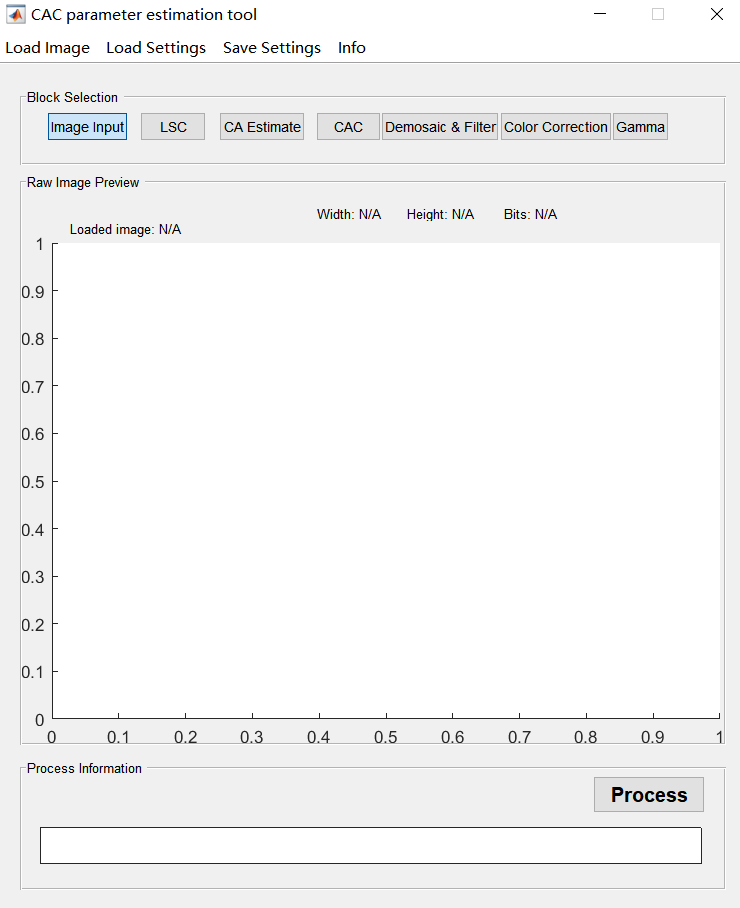
The specific operation steps are as follows:

1. Click the “Demosaic&Filter” button to set the bayer pattern format;

2. Click the “load image” button to load the RAW image, and the image will be displayed in the preview window;

3. Set the parameters under the “Demosaic&Filter” interface;

   Because the CAC module runs after demosaic, the tool first implements a simple demosaic function here.

   • ISP_demosaic_threshold: The default value of the threshold is set to 4. The higher the setting, the fewer edges the edge detection algorithm will detect; lower values will result in more edges being detected, and a value of 255 means edge detection is completely disabled.

   • Simulate 2 additional Line Buffers: Allows the user to extend the vertical offset. This allows the vertical vector clipping to be set to +-3. In this case, no chroma reduction filtering is performed, and it is unchecked by default.

   • Filter stage1 select:

   • Sharpen Level:

   • Denoise Level:

   • Lum_weight Off: Allows disabling a special feature of the filter algorithm. This feature helps suppress noise that is stronger in dark areas than in bright areas. Due to nonlinear gamma correction, in the processing chain, contrast and noise are emphasized in dark areas and attenuated in bright areas. To compensate for this, before comparing the texture parameter with the threshold, the texture parameter is weighted using a function derived from the average brightness of the 5x5 kernel. It is unchecked by default, and the image preview effect has less noise.

4. Click the “Color Correction” button to set the parameters under this interface;

   • Check “ISP_bls_enable” and set the correct BLC;

   • Check “Auto White-Balance”;

   • Set CCM;

   • The global gain default is set to 1.0.

5. Click the “Gamma” button to set the gamma curve, which defaults to gamma 2.2;

6. Click the “LSC” button, then click “Load parameters” to load the LSC calibration parameters under the corresponding light source D50, and check “Enable”;

7. Click the “CA Estimate” button, check the “CA_Estimate” box, and click “Process” to run;

8. Click the “CAC” button to view the calibration results from this interface.

Module Introduction

BLS

Function Description

Subtract the black level offset value to ensure linear consistency of the data.

Main Parameters

Parameter	Type and Value Range	Description
bls_enable	bool	BLS enable switch
bls	int bls[4] 0~4095	Black level compensation values for four channels, the set values are based on ISP 12bits

Debugging Strategy

Although it supports separate black level compensation values for the four channels, it is still recommended to use the same value.

LSC

Function Description

In K230, the LSC algorithm uses a 32x16 grid to calibrate the image. During RAW image data processing, the LSC algorithm divides the image into 32x16 sub-blocks and processes the four channels of the RAW image.

Main Parameters

Parameter	Type and Value Range	Description
enable	bool	LSC enable switch
matrix	matrix[4][1089]	Lens shading calibration parameters for the four channels R, Gr, Gb, B, obtained from the calibration file
x_size	xSize[32]	Distance between every two grid nodes on the x-axis, obtained from the calibration file
y_size	ySize[16]	Distance between every two grid nodes on the y-axis, obtained from the calibration file

Dgain

Function Description

The ISP digital gain is mainly used to enhance the brightness of the image.

Main Parameters

Parameter	Type and Value Range	Description
enable	bool	Enable switch for ISP digital gain
digital_gain_r	float 1.0~255.99	Digital gain for R channel
digital_gain_gr	float 1.0~255.99	Digital gain for Gr channel
digital_gain_gb	float 1.0~255.99	Digital gain for Gb channel
digital_gain_b	float 1.0~255.99	Digital gain for B channel

AE

Function Description

AE (Auto Exposure) controls image brightness. The main debugging of the AE module includes adjusting the brightness of the AE target value, and adjusting the AE convergence speed and smoothness.

Main Parameters

Parameter	Type and Value Range	Description
enable	bool	Auto exposure enable switch. false: Disable auto exposure true : Enable auto exposure
antiFlickerMode	Int 0~3	Anti-flicker working mode 0: Off 1: 50Hz 2: 60Hz 3: User defined
autoHdrEnable	bool	true: In HDR mode, automatically calculate the HDR ratio of the current frame false: In HDR mode, use a fixed HDR ratio
dampOver	float 0~1.0	Damping factor, used to smooth AE convergence during overexposure
dampOverGain	float 0~128.0	Convergence acceleration gain factor outside the clip range during AE overexposure, the larger the value, the faster the convergence
dampOverRatio	float 1.0~4.0	Ratio factor outside the clip range during AE overexposure, the smaller the value, the faster the convergence
dampUnder	float 0~1.0	Damping factor, used to smooth AE convergence during underexposure
dampUnderGain	float 0~16.0	Convergence acceleration gain factor outside the clip range during AE underexposure, the larger the value, the faster the convergence
dampUnderRatio	float 0~1.0	Clip range ratio factor during AE underexposure, the larger the value, the faster the convergence
expV2WindowWeight	float[32x32] 0~255	Exposure weight of each sub-block
frameCalEnable	bool	Exposure setting frame interval enable switch. true : Enable exposure setting frame interval function false: Disable exposure setting frame interval function
lowLightHdrGain	float[20] 0~255.0	In WDR mode, the gain value corresponding to the current gain level
lowLightHdrLevel	int 0~16	Total gain levels in WDR mode
lowLightHdrRepress	float[20] 0~1.0	In WDR mode, the target brightness suppression ratio corresponding to the current gain level
lowLightLinearGain	float[20] 0~255.0	In linear mode, the gain value corresponding to the current gain level
lowLightLinearLevel	int 0~19	Total gain levels in linear mode
lowLightLinearRepress	float[20] 0~1.0	In linear mode, the target brightness suppression ratio corresponding to the current gain level
motionFilter	float 0~1.0	Motion change smoothing parameter, used to calculate the motion factor in AE scene evaluation adaptive mode
motionThreshold	float 0~1.0	Motion discrimination threshold
roiNumber	int	Current ROI window index
roiWeight	float	Brightness calculation weight of the current ROI window
roiWindow	float (fx,fy,fw, fh)	Starting point coordinates (x,y) and width/height of the current ROI window
semMode	int 0~2	Scene mode 0: Scene evaluation disabled mode 1: Scene evaluation fixed mode 2: Scene evaluation dynamic mode
setPoint	float 0~255.0	Set the brightness target value of AE
targetFilter	float 0~1.0	AE brightness target value change smoothing coefficient, the larger the value, the faster the change
tolerance	float 0~100.0	Set the percentage lock range of AE brightness target value
wdrContrast.max	float 0~255.0	Maximum contrast value for calculating AE setpoint in AE scene evaluation adaptive mode
wdrContrast.min	float 0~255.0	Minimum contrast value for calculating AE setpoint in AE scene evaluation adaptive mode

AWB

Feature Description

Under different light source environments, the color presented by an object will vary. The human eye has the characteristic of color constancy and can recognize the true color of an object under different color temperature light sources. However, the sensor’s response to different light sources differs from that of the human eye, which will lead to color cast. AWB can reduce the influence of external light sources on the true color of an object, converting color-cast objects into objects with no color cast under ideal daylight light sources.

Main Parameters

Parameter	Type and Value Range	Description
enable	bool	true : Enable AWB false: Disable AWB
awbTempWeight	float 0.0~1.0	AWB color temperature light source weight
mode	int 0,1	0: AWB 1: AWB METEDATA
roiNumber	int	Current ROI window index
roiWeight	float	AWB calculation weight for the current ROI window
roiWindow	float (fx,fy,fw,fh)	Starting point coordinates (x,y) and width/height of the current ROI window
useCcMatrix	bool	true : Enable CCM adaptation false: Disable CCM adaptation
useCcOffset	bool	true : Enable CCM offset adaptation false: Disable CCM offset adaptation
useDamping	bool	true : Enable AWB damping variation false: Disable AWB damping variation
kFactor	float	Photosensitivity coefficient used to identify outdoor and transition intervals

Parameter kFactor Calibration Instructions

In the AWB algorithm, the environment is determined as outdoor if: Exp*kFactor <=0.12 (Exp is the exposure amount).

For example, taking 2000 lux as the dividing point of environmental illuminance between outdoor and transition, obtain the exposure value (ET * gain) corresponding to this illuminance, then it can be calculated: kFactor=0.12/(ET*gain).

The larger the kFactor, the stronger the sensitivity of the sensor; the smaller the kFactor, the weaker the sensitivity of the sensor.

The kFactor parameter is located in the AWB parameters of the xml file and needs to be calculated using the above method before being filled in.

WDR

Function Description

During image processing, it is easy to find that the image contrast is insufficient, and the details of the bright and dark areas may be lost. The WDR module uses the histogram statistical equalization method to enhance the image contrast, and at the same time enhance the details of the bright and dark areas.

Main Parameters

Parameter	Type and Value Range	Description
enable	bool	WDR enable switch
contrast	int -1023~1023	The larger the value, the stronger the local contrast
entropy	int[20]	local weight
entropy_base	int	Brightness factor parameter. The larger the base, the smaller the slope, and the stronger the local contrast
entropy_slope	int	Brightness factor parameter. The larger the base, the smaller the slope, and the stronger the local contrast
flat_strength	int 0~19	Stretching strength for flat areas
flat_thr	int 0~20	Flat area threshold. The larger the value, the flatter the image is judged. If it is less than the threshold, it is judged as a flat area; if it is greater than the threshold, it is judged as a texture area
gamma_down	int[20]	local weight
gamma_pre	int[20]	local weight
gamma_up	int[20]	global curve
global_strength	int 0~128	Global contrast strength
high_strength	int 0~128	Protection strength for bright area information in the image. The larger the value, the stronger the protection of the bright area information in the image
low_strength	int 0~255	Protection strength for dark area information in the image. The larger the value, the stronger the protection of the dark area information in the image
strength	int 0~128	Total strength

Debugging Strategy

In linear mode, Strength is fixed at 128. Low Strength is actually the maximum gain, which is used together with High Strength to adjust the image brightness. When the dark areas of the image need to be brightened, Low Strength can be increased. When the bright areas of the image are overexposed and need to be suppressed, High Strength can be increased. To avoid excessive enhancement of noise, as the gain increases, Low Strength should be gradually decreased, while High Strength can remain unchanged or gradually increased. Global Strength is used to control the overall contrast. When the overall contrast of the image is weak, this parameter can be appropriately increased. Contrast, Flat Strength, and Flat Threshold are used to adjust the local contrast. You can first use the default parameters. If the local contrast is not good, you can appropriately increase Contrast. Increasing the contrast can make the gray shadow in the flat area more obvious. Currently, adjust the Flat Threshold to identify the texture area and the flat area, and increase the Flat Strength to smooth the flat area to reduce the gray shadow.

GE

Function Description

The main function of Green Balance is to balance the difference between adjacent pixels Gr and Gb in RAW data, preventing patterns such as checkerboard or maze-like artifacts from occurring in subsequent demosaic interpolation algorithms. This module is located before DPCC.

Main Parameters

Parameter	Type and Value Range	Description
enable	bool	Enable switch for green balance
threshold	float 0~511.0	Green balance intensity threshold.

DPCC

功能描述

Due to limitations in sensor manufacturing processes, it is impossible for all pixels of a sensor with several million pixels to be intact, especially for lower-cost sensors, which may have more bad pixels. If bad pixels in the sensor are not processed early, they may be amplified and spread in subsequent demosaic interpolation algorithms. Therefore, this module performs calibration of bad pixels before the demosaic module. The fixed bad pixel table can accommodate a maximum of 2048 bad pixels. Seven sets of configuration values are available for selection.

主要参数

参数	类型及取值范围	描述
enable	bool	DPCC enable switch. false: Disable DPCC (Default); true: Enable DPCC
bpt_Enable	bool	Bad pixel table enable switch
bpt_Num	int 0~1024	Index of the current bad pixel in the bad pixel table
bpt_out_mode	int 0~14	Selection of median mode for calibration output of bad pixels in the bad pixel table
bpt_pos_X	int	Horizontal address of the bad pixel
bpt_pos_Y	int	Vertical address of the bad pixel
bypass	bool	DPCC bypass enable switch. false: Pass through DPCC true : Bypass DPCC
line_mad_fac	int lineMadFac[2][3] 0~63	Mean absolute difference factor
line_thresh	int lineThresh[2][3] 0~255	Line thresholds for R & B & G
methods_set	int methodsSet[3] 0~8191	Selection of bad pixel calibration methods enabled for each channel. There are two methods for bad pixel calibration, which can be divided into median filtering with the center point and median filtering without the center point according to the settings.
out_mode	int 0~15	Interpolation mode of the calibration unit
pg_fac	int pgFac[2][3] 0~63	Peak gradient factor
rg_fac	int rgFac[2][3] 0~63	Rank gradient factor
rnd_offs	int rndOffs[2][3] 0~3	Rank neighbor difference rank offset
rnd_thresh	int rndThresh[2][3] 0~63	Rank neighbor difference threshold
ro_limits	int roLimits[2][3] 0~3	Rank offset limit
set_use	int 1~7	Selection of which set of calibration values to use

DPF

Function Description

Bilateral filtering for noise reduction.

Main Parameters

Parameter	Type & Value Range	Description
enable	bool	Enable switch.
gain	float 1.0~1000.0	sensor gain
gradient	float 0.1~128	Gradient
min	float 1.0~128.0	strength clip
offset	float 0~128.0	The larger the value, the stronger the noise reduction
div	float 0~64.0	The larger the value, the weaker the noise reduction
sigma_g	float 1.0~128.0	Spatial filtering of G channel, the larger the value, the greater the weight
sigma_rb	float 1.0~128.0	Spatial filtering of R&B channel, the larger the value, the greater the weight
noise_curve	float 0~4095.0	17-point curve, obtained from calibration file

DNR

Feature Description

Image denoising is an important part and step in digital image processing, and the denoising effect will impact subsequent image processing. 3DNR combines temporal and spatial information to more effectively identify and reduce noise, and includes motion detection to ensure that the denoising process does not affect the detail and clarity of moving objects.

Main Parameters

Parameter	Type and Value Range	Description
enable	bool	Overall enable switch for 2DNR and 3DNR
tnr_en	bool	3DNR enable switch
nlm_en	bool	2DNR enable switch
sigma	float [0.1~16.0]	2DNR strength, the larger the value, the greater the denoising strength
strength	float 0~128.0	2DNR strength, the larger the value, the greater the denoising strength
blend_motion	float 0~100.0	Represents the weight of the 2DNR-processed frame and the tnr output frame. Changing it affects the denoising strength, but the motion estimation remains unchanged
blend_slope	float 0.1~32.0	Blend slope; the larger the value, the greater the weight of the NLM image. The weight slope of 2DNR blend. The smaller the value, the higher the static blend weight; the larger the value, the higher the motion blend weight.
blend_static	float 0~100.0	Represents the weight of the 2DNR-processed frame and the tnr output frame in static regions
dialte_h	float	Window width of 3DNR motion dilation
filter_len	float 0~1024	Temporal filtering window length, indicating how many frames of information are referenced
filter_len2	float 0~100	Length of motion history frames
motion_dilate_en	bool	motion_dilate enable switch
motion_erode_en	bool	motion_erode enable switch
noise_level	float 0~1024	Motion detection threshold, values greater than this are judged as motion areas
noisemodel_a	float	Slope of the custom pregamma curve
noisemodel_b	float	Offset value of the custom pregamma curve
pregamma_en	bool	pregamma transform enable switch
preweight	float	Weight of motion information from the previous frame
range_h	float	Radius of the motion detection window in the horizontal direction, 7 represents using 15x15
range_v	float	Radius of the motion detection window in the vertical direction, 7 represents using 15x15
sadweight	float	Sets the weight of motion difference type a, the final motion detection is a weighted sum of two types of motion differences, parameter for calculating block diff
thr_motion_slope	float	Transition section, beyond the slope is 100% motion area

Debugging Strategy

1. First enable tnr, nlm, dilate, erode, pregamma;

2. Set filter_len to control the damping ratio of the reference frame;

3. Set filter_len2 to control the damping ratio of the motion frame;

4. Use noise_level to distinguish foreground from background;

5. Set thr_motion_slope, sad weight, preweight to calculate the motion area.

Please note: When TNR is enabled, the ISP requires that the sensor/ISP Hblank cannot be less than 180 pixel clocks (recommended to set to 256 pixel clocks), and the Vblank should not be less than 60 sensor ET lines.

Demosaic

Function Description

The Demosaic module mainly implements the function of converting input Bayer format data into RGB format data through interpolation algorithms, while supporting denoising, sharpening, demoiré, and purple edge removal functions.

Main Parameters

Parameter	Type and Value Range	Description
demosaic_enable	bool	Demosaic enable switch
demosaic_thr	int 0~255	Interpolation threshold for R and B channels. Values below this threshold use non-directional interpolation
dmsc_dir_thr_min	int 0~4095	G channel interpolation in dark area
dmsc_dir_thr_max	int 0~4095	G channel interpolation in bright area
dmsc_denoise_strength	int 0~31	Low-frequency filter denoise strength
dmsc_sharpen_enable	bool	Sharpen enable switch
dmsc_sharpen_clip_black	int 0~2047	Black edge sharpen clip parameter
dmsc_sharpen_clip_white	int 0~2047	White edge sharpen clip parameter
dmsc_sharpen_factor_black	int 0~511	Sharpen enhancement for black edges. The larger the value, the more obvious the sharpen enhancement effect
dmsc_sharpen_factor_white	int 0~511	Sharpen enhancement for white edges. The larger the value, the more obvious the sharpen enhancement effect
dmsc_sharpen_line_enable	bool	Continuous line sharpen enhancement enable switch
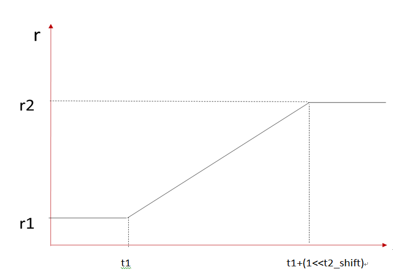
dmsc_sharpen_line_r1	int 0~255	r1 is the sharpen strength corresponding to value points less than thr
dmsc_sharpen_line_r2	int 0~255	r2 is the sharpen strength corresponding to value points greater than (thr + (1<<thr_shift1))
dmsc_sharpen_line_strength	int 0~4095	The larger the value, the greater the line sharpen strength
dmsc_sharpen_line_thr	int	Line sharpen threshold
dmsc_sharpen_line_thr_shift1	int 0~10	/
dmsc_sharpen_r1	int 0~256	Sharpen curve parameter
dmsc_sharpen_r2	int 0~256	Sharpen curve parameter
dmsc_sharpen_r3	int 0~256	Sharpen curve parameter
dmsc_sharpen_size	int 0~16	Represents the presentation of high-frequency signals. The smaller the value, the more details in the sharpen area, and more small details will be sharpened
dmsc_sharpen_t1	int 0~2047	Sharpen curve parameter, value point t1
dmsc_sharpen_t2_shift	int 0~11	Sharpen curve parameter, value point (t1+(1<<t2_shift))
dmsc_sharpen_t3	int 0~2047	Sharpen curve parameter, value point t3
dmsc_sharpen_t4_shift	int 0~11	Sharpen curve parameter, value point (t3+(1<<t4_shift))
dmsc_demoire_area_thr	int 0~32	Demoiré area threshold. Demoiré processing is performed only on areas greater than the threshold
dmsc_demoire_enable	bool	Demoiré enable switch
dmsc_demoire_r1	int 0~255	Demoiré strength curve parameter, r1 is the correction strength corresponding to value points less than t1
dmsc_demoire_r2	int 0~255	Demoiré strength curve parameter, r2 is the correction strength corresponding to value points greater than (t1 + (1<<t2_shift))
dmsc_demoire_t1	int 0~255	Demoiré strength curve parameter, value point t1
dmsc_demoire_t2_shift	int 0~8	Demoiré strength curve parameter, value point (t1 + (1<<t2_shift))
demoire_edge_r1	int 0~255	Demoiré conversion curve parameter, r1 is the moiré rate corresponding to value points less than t1
demoire_edge_r2	int 0~255	Demoiré conversion curve parameter, r2 is the moiré rate corresponding to value points greater than (t1 + (1<<t2_shift))
demoire_edge_t1	int 0~511	Demoiré conversion curve parameter, value point t1
demoire_edge_t2_shift	int 0~9	Demoiré conversion curve parameter, value point (t1 + (1<<t2_shift))
dmsc_demoire_sat_shrink	int 0~32	The larger the value, the stronger the saturation reduction in the moiré area
dmsc_depurple_cbcr_mode	int [0,1,2,3]	Depurple channel mode. 0: disable depurple, 1: R channel depurple, 2: B channel depurple, 3: R&B channel depurple
dmsc_depurple_enable	bool	Depurple enable switch
dmsc_depurple_sat_shrink	int 0~8	Saturation reduction value for purple edge area. The larger the value, the stronger the saturation reduction
dmsc_depurple_thr	int 8~255	Intensity threshold for detecting purple edges. The smaller the value, the more pixels are considered as purple fringes

Debugging Strategy

1. Interpolation

   For 12bit raw, the value 0 corresponds to the interpolation threshold dir_thr_min, the value 4095 corresponds to the interpolation threshold dir_thr_max, and the value in the middle corresponds to the corresponding value point on the line segment determined by dir_thr_min and dir_thr_max.

   

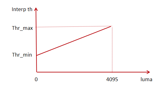
   Setting of demosaic_thr: gradient difference > threshold, directional interpolation; gradient difference < threshold, average interpolation. A smaller value means more false colors in high-frequency areas.

2. Sharpening and Denoising

   denoise_strength represents the low-frequency noise filter strength. When set to 0, it is equivalent to disabling the denoise function. Generally, the denoise function is disabled in the demosaic module, and it is only used here when the image noise is particularly large.

   Setting of sharpen curve parameters: the steeper the curve, the greater the sharpen strength.

   

   Setting of sharpen_line: when the image noise is relatively large, if you want the edges to be smoother and more continuous, you can enable sharpen_line. The basic effect of sharpen_line is to smooth lines or textures in the vertical or horizontal direction. The larger the vertical axis values sharpen_line_r1 and sharpen_line_r2, the closer the sharpen result is to directional (horizontal or vertical) enhancement. In addition, more points are wrongly connected, which may cause errors in high-frequency details.

   Setting of sharpen_factor&clip: the larger the factor value, the stronger the sharpen effect; the larger the clip value, the weaker the clipping effect and the more details are preserved. The setting of factor>clip should be avoided as much as possible, which keeps fewer black and white details but with high sharpen strength, resulting in a lack of layering.

3. Demoiré

   Demoiré conversion curve:

   

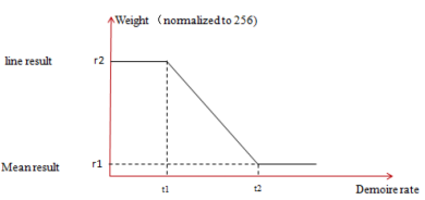
   Demoiré calibration curve:

   

ManualWB

Functional Description

Manually set the gain value of white balance.

Main Parameters

Parameter	Type and Value Range	Description
driver_load	bool	Indicates whether to load parameters under this module
gain	float [4] 1.0~3.999	White balance gain values for four channels

CCM

Function Description

Complete linear correction of color space through a standard 3×3 matrix and vector offset. CCM’s 3x3 matrix converts the sensor’s color space to the sRGB standard color space.

Main Parameters

Parameter	Type and Value Range	Description
enable	bool	CCM Switch
ccmatrix	float ccMatrix[9] -8.0~7.996	Color Calibration Matrix
ccoffset	ccOffset[3] -2048~2047(12bit)	Offset

Gamma

Function Description

The Gamma module mainly performs nonlinear transformation on the luminance space to adapt to general output devices.

Main Parameters

Parameter	Type and Value Range	Description
enable	bool	gamma enable switch
standard	bool	standard gamma enable switch
standard_val	float	gamma value, default 2.2
curve	int [64]	gamma curve of 64 points

Debugging Strategy

The default value of gamma 2.2 is used, and users can customize the gamma curve as needed.

EE

功能描述

The EE module is used for sharpening and enhancing image detail textures, achieving an improvement in image clarity. While sharpening image edges, it also controls relevant parameters and can suppress black and white edges in the image.

主要参数

参数	类型及取值范围	描述
enable	bool	EE功能的使能控制
ee_strength	int 0~128	EE强度
ee_src_strength	int 0~255	值越大，降噪强度越大。默认设为1
ee_y_up_gain	int 0~10000	亮边的gain强度
ee_y_down_gain	int 0~10000	暗边的gain强度
ee_uv_gain	int 0~1024	对边缘色彩饱和度的控制，值越大，饱和度下降越明显
ee_edge_gain	int 0~10000	对边缘细节的检测强度。gain值越大，检测到的边缘细节越多

CA

Function Description

The CA module adjusts image saturation based on the UV gain curve. Its main function is to eliminate color noise in dark areas or low-saturation areas. In practical applications, it can help eliminate false colors caused by the non-linearity of the R/G/B three channels in highlight overexposed areas and white balance deviation in low-saturation areas.

Main Parameters

Parameter	Type and Value Range	Description
ca_en	bool	Enable switch for the CA module
curve_en	bool	Enable switch for ca_curve and dci_curve
ca_mode	int [0,1,2]	0: Adjust saturation based on brightness; 1: Adjust saturation based on original saturation; 2: Adjust saturation based on both brightness and original saturation
ca_curve	flaot	ca curve with 64 points

DCI

功能描述

Dynamic Contrast Improve is used to adjust the global contrast of an image.

主要参数

参数	类型及取值范围	描述
dci_en	bool	dci使能开关
dci_curve	float	64个点的dci曲线

CProcess(Color Processing)

功能描述

在YUV域对图像的颜色进行处理。

主要参数

参数	类型及取值范围	描述
enable	bool	CProcess使能开关
luma_in	int	luminance input range。0: Y_in range [64..940]，1: Y_in full range [0..1023]
luma_out	int	luminance output clipping range。0: Y_out clipping range [16..235]，1: Y_out clipping range [0..255]
chroma_out	int	chrominance pixel clipping range at output。0: CbCr_out clipping range [16..240]，1: Full UV_out clipping range [0..255]
bright	float -128~127	亮度调整值
contrast	float 0.3~1.9921875	对比度调整值
hue	float -90~89	色调调整值
saturation	float 0~1.9921875	饱和度调整值

Compand

Function Description

Data compression and expansion module. Can be used for data compression and expansion processing.

Main Parameters

Parameter	Type and Value Range	Description
enable	bool	Data compression and expansion enable switch
compress_enable	bool	Data compression enable switch
compress_curve_x	int[64] 0~31	Data compression x-axis distance curve
compress_use_out_y_curve	bool	Data compression output Y-axis curve enable switch
compress_curve_y	int[64] 0~16777216	Data compression y-axis value curve
expand_enable	bool	Data expansion enable switch
expand_curve_x	int[64] 0~31	Data expansion x-axis distance curve
expand_use_out_y_curve	bool	Data expansion output Y-axis curve enable switch
expand_curve_y	int[64] 0~16777216	Data expansion y-axis value curve

CAC (Chromatic Aberration Correction)

Function Description

This module is used for chromatic aberration correction.

Main Parameters

Parameter	Type and Value Range	Description
a_blue	float -16~15.9375	Radial blue shift calculation parameter, calculated according to the formula (a_blue * r + b_blue * r^2 + c_clue * r^3)
a_red	float -16~15.9375	Radial red shift calculation parameter, calculated according to the formula (a_red * r + b_red * r^2 + c_red * r^3)
b_blue	float -16~15.9375	Radial blue shift calculation parameter, calculated according to the formula (a_blue * r + b_blue * r^2 + c_clue * r^3)
b_red	float -16~15.9375	Radial red shift calculation parameter, calculated according to the formula (a_red * r + b_red * r^2 + c_red * r^3)
c_blue	float -16~15.9375	Radial blue shift calculation parameter, calculated according to the formula (a_blue * r + b_blue * r^2 + c_clue * r^3)
c_red	float -16~15.9375	Radial red shift calculation parameter, calculated according to the formula (a_red * r + b_red * r^2 + c_red * r^3)
cac_enable	bool	CAC enable switch
center_h_offs	int	Horizontal distance between image center and optical center
center_v_offs	int	Vertical distance between image center and optical center

a_blue, b_blue, c_blue can be obtained from the blue_parameters of the CAC field in the xml file; a_red, b_red, c_red can be obtained from the red_parameters of the CAC field in the xml file; center_h_offs can be obtained from the x_offset of the CAC field in the xml file; center_v_offs can be obtained from the y_offset of the CAC field in the xml file.