FFT Routine#

What is FFT?#

FFT (Fast Fourier Transform) is an efficient algorithm used to convert a signal from the time domain to the frequency domain, thereby analyzing the frequency components contained in the signal and their amplitudes. In other words, FFT tells us:

What frequencies are present in the signal
The intensity (amplitude) corresponding to each frequency

FFT is widely applied in:

Audio spectrum analysis (such as music visualization)
Image frequency analysis (such as filtering)
Communication systems (modulation, demodulation)
Vibration analysis, radar signal processing

FFT Usage Example#

This example first synthesizes a known composite signal, then uses FFT to analyze it, visually demonstrating the correspondence between the time-domain waveform and the frequency-domain spectrum.

Import Necessary Modules#

import ulab
from ulab import numpy as np
import math

Synthesize Composite Signal#

The mathematical expression of a sine wave is usually represented as:

\[ y(t) = A \cdot \sin(2\pi f t + \phi) \]

Where the meanings are as follows:

$A$: Amplitude — the height of the peak;
$f$: Frequency — the number of oscillations per second, in Hz;
$t$: Time;
$\phi$: Phase — the initial offset of the waveform, in radians;
$2\pi f$: Angular frequency — in rad/s.

In embedded systems, floating-point computation (especially double precision) is costly, so fixed-point numbers are commonly used for computation.

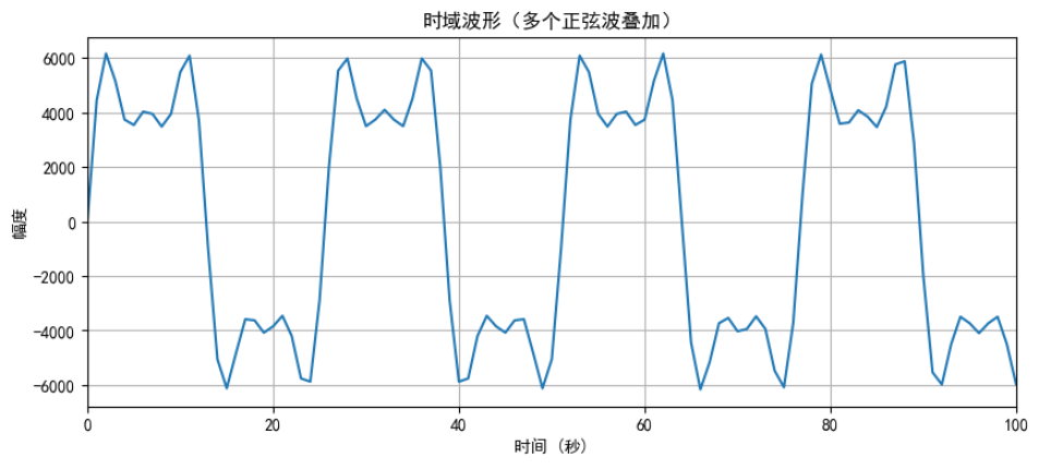
The following code synthesizes a signal composed of a 50 Hz fundamental frequency and its 3rd harmonic (150 Hz) and 5th harmonic (250 Hz), with decreasing amplitudes.

fs = 1280       # Sampling rate
duration = 1     # Seconds
amplitude = 32767 # Maximum amplitude for fixed-point (int16)
N = 128  # FFT points

n_samples = int(fs * duration)
# Create an array from 0 to n_samples-1
n = np.arange(n_samples, dtype=np.int16)

# Set three fundamental frequencies
f1, f2, f3 = 50, 150, 250

# Generate three sine waves
sin_f1 = np.sin(2 * math.pi * f1 * n / fs)/3
sin_f2 = np.sin(2 * math.pi * f2 * n / fs)/3
sin_f3 = np.sin(2 * math.pi * f3 * n / fs)/3

# Combine waveforms
signal = amplitude * 0.5 * sin_f1 + amplitude * 0.25 * sin_f2 + amplitude * 0.125 * sin_f3

# Convert floating-point results to int16 type
signal_fixed = np.zeros(len(signal), dtype=np.int16)
for i in range(len(signal)):
    signal_fixed[i] = int(signal[i])

# Print the first 20 sample points
print(signal_fixed[0:20])

Synthesized waveform diagram: Origal Waveform

FFT Analysis#

Use the K230’s FFT hardware module to analyze the signal:

# N is the number of FFT points, 0x555 is the hardware scaling factor (recommended default value)
fft = FFT(signal_fixed, N, 0x555)
res = fft.run()

amps = fft.amplitude(res)  # Get the amplitude of each frequency point
print(amps)

freqs = fft.freq(N, 1280)  # Get the frequency values of all frequency points
print(freqs)

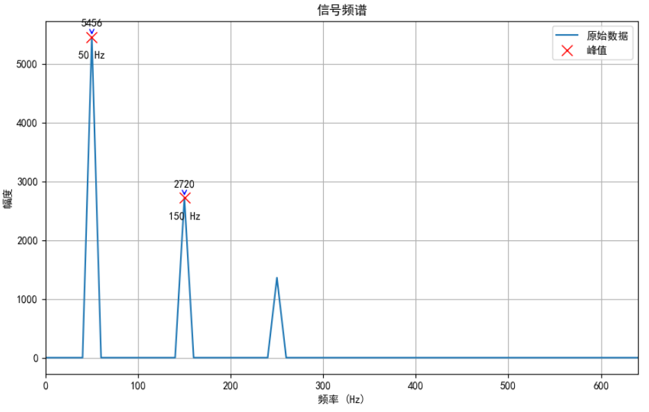
The spectrum result is shown in the figure below. It can be seen that there are significant peaks at 50 Hz, 150 Hz, and 250 Hz, and the amplitude ratio is approximately 4:2:1, consistent with the settings during signal synthesis. FFT waveform

Frequency Resolution Δf#

The number of FFT points $N$ represents the number of sampling points used in a single transform, frequency resolution is:

\[ \Delta f = \frac{f_s}{N} \]

where $f_s$ is the sampling rate.

For example, when $f_s = 16,\text{kHz}$:

FFT Points	Time Window Length (ms)	Frequency Resolution Δf (Hz)
64	4.0	250
128	8.0	125
256	16.0	62.5

Explanation:

The larger N, the smaller Δf, and the higher the frequency resolution
The smaller N, the higher the time resolution, which is more suitable for capturing transient signals

⚠ Notes#

Item	Description
Sampling Rate	Affects the maximum frequency you can detect (only up to `half the sampling rate`, known as the Nyquist frequency)
Signal Length	FFT output frequency resolution = sampling rate / signal length
Complex Results	FFT output is complex, usually taking its magnitude to represent energy
Normalization	The output amplitude often needs to be multiplied by certain coefficients (such as `2 / N`) for normalization

FFT Routine

Contents